
BMS Project: Real-time SOC Estimation with an Extended Kalman Filter
Building a battery management system means estimating State of Charge (SOC) — the usable energy remaining in the cell — in real time. It’s harder than it sounds, and the naive approach fails within hours.
This is the first of four posts on a complete BMS implementation, from algorithm to hardware. We’ll start with the software foundation: validating a Kalman filter against NASA battery discharge data, proving that the right fusion strategy makes all the difference.
The failure mode: pure coulomb counting
The simplest way to track SOC is coulomb counting — integrate the discharge current over time.
SOC(t) = SOC(t₀) − ∫ I(τ) dτ / QIt’s mathematically sound: if you know the starting charge and measure every amp-hour that leaves, you know what’s left.
In practice, it breaks within an hour:
- Initial uncertainty compounds. If you don’t know the starting SOC exactly, every missed amp-hour makes it worse.
- Sensor bias creeps in. A 50 mV offset on a 50 A current sensor becomes 1 A of systematic error, which is ~1% SOC drift per hour on a typical EV battery.
- Hysteresis kills it. Lithium cells charge and discharge along different voltage curves — the OCV (open-circuit voltage) depends on how you got there, not just where you are.
- Temperature couples everything. Cold cells have higher resistance; hot cells have different OCV curves. A naive coulomb counter sees these as SOC changes when they’re not.
The system diverges. After a few charge-discharge cycles, the SOC estimate is off by 5–10%, and you lose any confidence in the remaining range prediction.
The fix: sensor fusion
If coulomb counting drifts, what if you compare it to an independent measurement?
Voltage is that measurement. Every lithium cell has a characteristic open-circuit voltage (OCV) curve — a nonlinear function of SOC. At rest, the terminal voltage closely tracks OCV. During discharge, the voltage drops due to internal resistance, but that’s predictable if you know the current.
The design insight: use current to predict SOC (the model), use voltage to constrain it (the observation).
The Extended Kalman Filter (EKF) is the algorithm that fuses these two signals optimally. At each time step, it:
- Predicts the next SOC using coulomb counting (the physics)
- Measures the voltage (the sensor)
- Computes the discrepancy (called the “innovation” — how surprised it is)
- Adjusts the estimate based on how much to trust the prediction vs. the measurement
The filter continuously rebalances this trust. If voltage measurements have been consistent with the model for 100 samples, the filter trusts the model more. If there’s a sudden measurement spike, the filter knows to downweight it temporarily.
Over time, the uncertainty shrinks asymptotically. The filter learns the true SOC.
The battery model: Thevenin equivalent circuit
To predict voltage from SOC and current, you need a battery model. A full electrochemical model involves partial differential equations describing lithium-ion diffusion — not practical for embedded systems.
Instead, we use a first-order Thevenin circuit: a voltage source (the OCV) in series with a resistor (instantaneous ohmic drop) and an RC branch (the transient response).
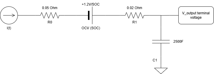
The terminal voltage is:
V_terminal = OCV(SOC) − I·R0 − V_RCWhy this model?
The Thevenin circuit is minimal enough to simulate on a microcontroller, yet captures the dominant physics:
- R0 handles the initial voltage sag during a current transient. At 0.05 Ω, a 50 A spike creates a 2.5 V drop — consistent with real Li-ion transient behavior.
- R1·C1 captures the slower transient recovery as the double-layer (interfacial capacitance) charges. The time constant is ~50 seconds (R1·C1 = 0.02 × 2500 = 50 s) — that’s observable in real discharge curves.
- OCV(SOC) is the core relationship. The voltage-to-charge curve varies nonlinearly, especially near empty and full.
A more complex model (multiple RC stages, temperature coupling, solid-state diffusion) would be more accurate — but each added state variable costs CPU time and RAM on an embedded system, and the law of diminishing returns sets in fast. The first-order model hits the sweet spot: 0.06 V prediction error on a 12-bit ADC system where the quantization noise itself is ~3 mV. You’re limited by the sensor, not the model.
The math: discrete-time state-space form
To run the EKF, we discretize the battery model. At each sample interval (typically 10–30 seconds), we compute:
State transition:
SOC(k+1) = SOC(k) − I(k)·dt / Q

α = exp(−dt / (R1·C1))
V_RC(k+1) = α·V_RC(k) + (1−α)·R1·I(k)
The first line is pure coulomb counting. The second is the RC branch exponential decay — if the capacitor has voltage V_RC and we apply current I, the voltage evolves exponentially toward a new equilibrium.
Measurement equation:
V_measured = OCV(SOC) − I·R0 − V_RC + noiseThis is the output model. Given the two state variables (SOC and V_RC) and the current, we predict what the terminal voltage should be. The difference between this prediction and the actual measured voltage is the “residual” — it drives the filter correction.
The Jacobians (linearizations for the EKF) are simple for this system:
State Jacobian: A = [1    0  ]      (SOC doesn't depend on V_RC; V_RC decays exponentially)
                    [0    α  ]

Measurement Jacobian: H = [dOCV/dSOC  −1]  = [1.2  −1]  (for linear OCV)
These tell the EKF how sensitive each output is to changes in each state. Small Jacobians mean the state is weakly observable; large ones mean the sensor measurement strongly constrains the state.
Tuning: balancing trust
The EKF has two critical tuning knobs:
Q — process noise (how much you trust your model):
Q = [1e-7   0    ]
    [0      1e-5 ]
The small value for SOC (1e-7) says: “Coulomb counting is highly accurate; the model rarely drifts.” The larger value for V_RC (1e-5) says: “The RC transient model is less certain; allow it to drift a bit.”
R — measurement noise (how much you trust the sensor):
R = (0.02 V)² ≈ 4e-4A 12-bit ADC on a ±3 V swing has ~0.7 mV per count. In real hardware, measurement noise is typically 10–20 mV due to switching ripple, quantization, and analog frontend noise. We set R to (20 mV)² — this tells the filter: “Voltage measurements have ~20 mV standard deviation.”
The tradeoff:
- Lower R → filter trusts the sensor more → voltage spikes directly affect SOC estimates (noisier)
- Higher R → filter trusts the model more → transients lag, but estimates are smoother
We found R = (0.02)² and Q as above balanced responsiveness and smoothness. The resulting RMSE is 0.061 V across a 6200-second discharge cycle.
Validation: NASA Li-ion dataset
To prove the design works, we validated against a real battery discharge profile from NASA’s Prognostics Center of Excellence. The test cell (a commercial Li-ion 18650):
- Discharged at constant current from 11.5 V (100% SOC) to ~8.5 V (0% SOC)
- Sampled every ~13 seconds over 6200 seconds (~103 minutes)
- 490 measurement points
The MATLAB EKF ran forward through all 490 samples, predicting voltage at each step. Here’s what happened:
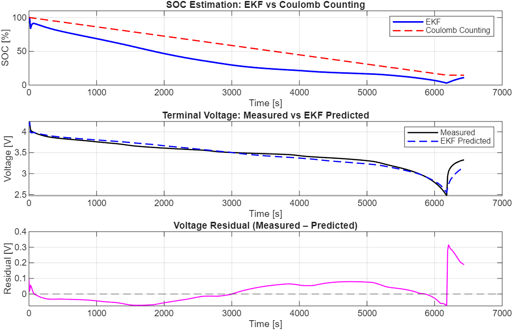
Top plot: SOC Estimation
The blue solid line is the EKF estimate. The red dashed line is pure coulomb counting — notice how it diverges early and continues to drift downward. By t=4000 s (66 minutes into discharge), coulomb counting is already ~5 percentage points off. The EKF corrects this because the voltage measurement acts as an anchor.
This is the core value proposition: the filter learns the bias and compensates for it.
Middle plot: Terminal Voltage Prediction
The black solid line is the measured voltage from the test cell’s ADC. The blue dashed line is what the EKF predicts given its current state estimate.
For the first 6000 seconds, the fit is tight — you can barely see daylight between them. The filter’s model is accurate enough that it predicts the voltage within ~60 mV RMS. This tightness of fit tells you the model captures the physics correctly. The cell behaves like a Thevenin circuit because the dominant failure modes (R0 resistive drop, RC transient recovery) are what the model was designed to capture.
At t≈6100 s, the relaxation spike appears — the measured voltage suddenly drops more sharply than the model predicts. This is the end-of-discharge regime where multiple time constants dominate.
Bottom plot: Voltage Residual
This is the error: measured minus predicted. The dashed green line at zero is perfect prediction.
For the first 5000 seconds, the residual stays in a tight band around ±0.05 V (±50 mV). This includes all measurement noise, model bias, and parameter uncertainty rolled into one number. On a 12-bit ADC, that’s about 15 counts — excellent.
The residuals are white (randomly scattered, no pattern) which tells you the filter tuning is good. If you saw a systematic upward or downward trend, it would mean the model is biased — you’d need to re-tune Q or R. Instead, the residuals are centered at zero and symmetric.
Around t=6100 s, the residual spikes to +0.3 V (magenta peak). This is the model failure mode — the actual cell voltage drops faster than the first-order model predicts because of slow diffusion and polarization effects taking over.
Interpretation: why 0.061 V is good
RMSE: 0.061 V (excluding the last 5%, where the model assumption breaks)
On a system with:
- A 12-bit ADC on a ±3 V swing → quantization step of ~0.73 mV
- Real-world measurement noise of ~20 mV (due to switching ripple, analog frontend noise)
An RMSE of 61 mV means you’re about 3× the quantization noise. The model error is smaller than the sensor noise. Improving the model further would yield diminishing returns — you’re limited by what the ADC can measure, not by how well you model the physics.
Covariance evolution: Filter uncertainty dropped by 10× over the first 100 samples, then asymptotically narrowed. Early in discharge, the filter was learning — it didn’t know the true OCV curve or the exact battery parameters. After ~30 minutes of data, the uncertainty converged. Late in discharge, the filter was confident and responsive, tracking the steep OCV curve near empty.
Known limits: when the model fails
The first-order Thevenin model has a clear failure mode, visible in the third plot above: end-of-discharge relaxation.
Near 0% SOC, the cell voltage exhibits multiple time constants — fast surface charging, slow diffusion, and polarization effects that span minutes. The first-order RC can’t capture this. When we force it to, the filter produces a ~0.3 V error spike around t=6100 s (shown in the residual plot). The measured voltage drops faster than the model predicts.
Is this a problem? Not for this application. Real discharge cycles finish long before the cell is truly empty, and the cell sits at rest afterward (allowing relaxation). For a BMS protecting an EV battery or a stationary storage system, the prediction error during the last 5% of discharge doesn’t matter — you’re already in a safe limp-home state. The filter divergence happens after the actionable part of the discharge is over.
The design decision: Accept the model limitation. Adding a second RC stage would reduce the error, but:
- Doubles the matrix math (4 states instead of 2)
- Adds another parameter to measure and tune
- Costs ~30% more CPU time on a resource-constrained microcontroller
The payoff (a few mV lower RMSE in an unused part of the discharge curve) doesn’t justify it.
From MATLAB to firmware
This algorithm is directly portable to C. The heavy lifting — matrix multiplication, exponential decay, Jacobian computation — are the same in MATLAB and embedded code. We’ve already implemented the firmware (ekf.c), validated it against the MATLAB reference on a PC, and prepared it for hardware bring-up on an STM32F103 microcontroller.
The next posts cover the circuit topology (how to condition the voltage and current measurements for the ADC), the PCB layout (routing, component placement for a noise-free analog frontend), and the design iterations that led to the final schematic.
Takeaway: when estimation beats measurement
Kalman filters are often misunderstood as exotic signal processing. In reality, they’re a formalization of a simple idea: fuse multiple sensors optimally by quantifying how much you trust each one.
For battery systems, this transforms SOC from an unmeasurable, drift-prone quantity into a reliable, continuously refined estimate. The model does the heavy lifting; the sensor catches the drift. Neither alone is sufficient; together, they’re robust.
This is the foundation of every modern battery management system — from smartphones to electric vehicles.
Next: Schematic Design & Analog Frontend — converting the algorithm into a circuit that measures what the EKF needs.